Till the end 19th century, when electrical science research were on peak, different pioneer came up with analysis that a charged body moving will gain mass.
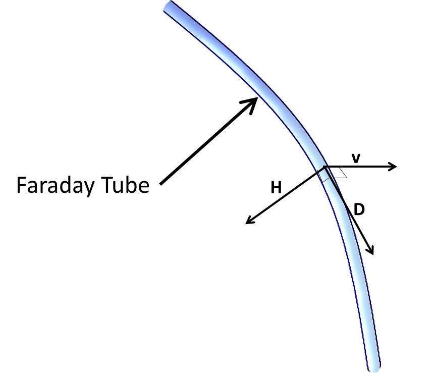
J J Thomson was the first to come up with the idea of increase of mass of moving charged body when moving in space. Most electrical pioneers were mostly mathematical with very hotchpotch physical theory. Faraday tubes are cylindrical vortex filaments extending from one atom to another.
He made quantized electricity in to “physical” entity with once single concept called Faraday Tubes, which itself extends from the actual works of Faraday.
He rejected Maxwell’s mathematical theory and took a physical approach, through empirically same as that of Maxwell. But different physical meaning.
He was the first to reject magnetic field, making it as a side effect of electric field in motion. In other words he brought physical unification of electricity and magnetism, unlike Maxwell’s mathematical unification.
His visualization of mass and momentum is different than that of Newtonian. For example, it’s assumed that mass is something resides inside an object. But according to Thomson, the mass is not just inside a charged object but rather extends throughout the space. Hence its motion leads to resistance hence appears like increase in apparent mass. This so-called relativistic mass increase has it’s roots in Thomson, and Not Einstein.
He showed that magnetic field is due to motion of faraday tubes. Hence:
He treated electric lines of force as not just abstract mathematical representations rather concrete physical reality as Faraday Tube of Induction. The displacement vector D is the abstract representation of number of excessive tubes passing per unit area in space between two points. And the net charge Q is the net effective Faraday tubes attached to a charged object.
So now you cannot have infinite number of lines of forces. Hence you cannot have fractional charge too, which electrolysis also confirms. Hence electricity is quantized in this manner, which can be traced to Thomson only.
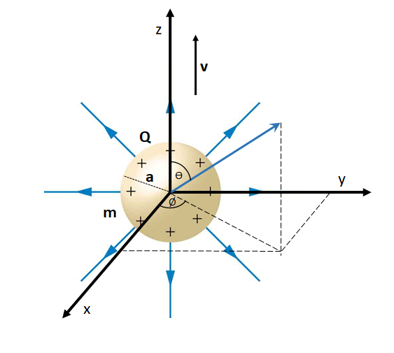
Lets have a charged sphere with radius a moving with velocity v, with surface charge Q in the origin has the electric field intensity E at any point of space in spherical coordinate system. It’s given by the expression:
\begin{equation}\begin{aligned}\large \overrightarrow{H}& =\overrightarrow{v} \times\overrightarrow{D} \\& = vD\sin\theta \\& = v \epsilon E\sin\theta \end{aligned}\end{equation}
Hence, from eqn(2) and eqn(3), we have:
\begin{equation}\begin{aligned}\large H = \frac{v Q \sin\theta}{4\pi r^{2}}\end{aligned}\end{equation}
The kinetic energy of the moving sphere is the net magnetic energy per unit volume in the system, which is given as:
Hence the apparent mass of the object appears to increase by the factor of \frac{\mu}{2\pi}\frac{Q^{2}}{3a}This is for velocity if the speed is very less compared to that of speed of light. As we haven’t taken the electric field intensity E distortion in higher speed, just magnetic field due to motion of tubes.
In next, will do much deeper analysis considering the field distortion with potential and momentum due to motion of tubes.
Now we will take a much deeper and detailed analysis for a charged body on how it’s electric field distorts based on speed as first devised by J J Thomson.
The magnetic energy per unit volume of the system is given as:
\begin{align*} \large So, \:\overrightarrow{E_{1}}=\overrightarrow{B} \times \overrightarrow{v}\end{align*}
This is the electric field intensity due to motional charge. Let’s call it E1 . Let’s E2 be the electric field in space due to the electric scalar potential Φ. Such that:
To find the constant A, we need to first find gradient of the scalar potential Φ and find the Displacement D, and then integrate the Displacement over entire surface of the sphere and equate with the net charge Q as per Gauss law.
Now according to Gauss law of electrostatics, the total electric displacement across a surface of a charged object is always the amount of charge contained.
\begin{align*} \large Q &= \large \frac{\epsilon A c^{2}}{(c^{2}-v^{2}_{z})}\oiint(\frac{x\hat{i}+y\hat{j}+z\hat{k}}{(x^{2}+y^{2}+(\frac{c^{2}}{c^{2}-v_{z}^{2}})z^{2})^{\frac{3}{2}}}).(\frac{x}{a}\hat{i}+\frac{y}{a}\hat{j}+\frac{z}{a}\hat{k})dS \\
&= \large \frac{\epsilon A c^{2}}{a(c^{2}-v^{2}_{z})}\oiint\frac{x^{2}+y^{2}+z^{2}}{(x^{2}+y^{2}+(\frac{c^{2}}{c^{2}-v_{z}^{2}})z^{2})^{\frac{3}{2}}}dS \\ &= \large \frac{\epsilon a A c^{2}}{(c^{2}-v^{2}_{z})}\oiint\frac{dS}{(x^{2}+y^{2}+(\frac{c^{2}}{c^{2}-v_{z}^{2}})z^{2})^{\frac{3}{2}}} \:\:\:\:\:\:\:\:\:\:\:\: \small[as, x^{2}+y^{2}+z^{2}=a^{2}]\end{align*}
\begin{align*} \small Q &= \small \frac{\epsilon A c^{2}}{(c^{2}-v^{2}_{z})}\oiint(\tiny \frac{x\hat{i}+y\hat{j}+z\hat{k}}{(x^{2}+y^{2}+(\frac{c^{2}}{c^{2}-v_{z}^{2}})z^{2})^{\frac{3}{2}}}).(\frac{x}{a}\hat{i}+\frac{y}{a}\hat{j}+\frac{z}{a}\hat{k} \small )dS \\
&= \small \frac{\epsilon A c^{2}}{a(c^{2}-v^{2}_{z})}\oiint\frac{x^{2}+y^{2}+z^{2}}{(x^{2}+y^{2}+(\frac{c^{2}}{c^{2}-v_{z}^{2}})z^{2})^{\frac{3}{2}}}dS \\ &= \small \frac{\epsilon a A c^{2}}{(c^{2}-v^{2}_{z})}\oiint\frac{dS}{(x^{2}+y^{2}+(\frac{c^{2}}{c^{2}-v_{z}^{2}})z^{2})^{\frac{3}{2}}} \\ & \large [as, x^{2}+y^{2}+z^{2}=a^{2}]\end{align*}
Now for proper evaluation, we need to convert this to spherical coordinate.So we have:\large x = rcos\phi sin\theta \\
\large y = rsin\phi sin\theta \\
\large z = rcos\theta \\
\large dS = r^{2}sin\theta d\theta d\phi
The variable r should be set to radius a as we are not integrating over volume.
So now putting the above expression into the integral we get:
Now we solve this integral by substituting:\frac{v_{z}}{\sqrt{c^{2}-v_{z}^{2}}}cos\theta = tan\psi \\
Hence,\: \frac{-v_{z}}{\sqrt{c^{2}-v_{z}^{2}}}sin\theta\: \partial\theta = sec^{2}\psi \: \partial \psi
Now the above integral becomes:\begin{align*} Q &= \large \frac{2 \pi\epsilon A c^{2}}{(c^{2}-v^{2}_{z})}\int_{tan^{-1}\frac{v_{z}}{\sqrt{c^{2}-v_{z}^{2}}}}^{tan^{-1}\frac{-v_{z}}{\sqrt{c^{2}-v_{z}^{2}}}}\frac{-\sqrt{c^{2}-v_{z}^{2}}}{v_{z}} \frac{sec^{2}\psi}{(1+tan^{2}\psi)^{\frac{3}{2}}} \: \partial \psi \\
&= \large \frac{-2 \pi\epsilon A c^{2}}{v_{z}\sqrt{c^{2}-v_{z}^{2}}}\int_{tan^{-1}\frac{v_{z}}{\sqrt{c^{2}-v_{z}^{2}}}}^{tan^{-1}\frac{-v_{z}}{\sqrt{c^{2}-v_{z}^{2}}}}cos \psi \: \partial \psi \\
&= \large \frac{-2 \pi\epsilon A c^{2}}{v_{z}\sqrt{c^{2}-v_{z}^{2}}}\left[ sin \psi \right]^{tan^{-1}\frac{-v_{z}}{\sqrt{c^{2}-v_{z}^{2}}}}_{tan^{-1}\frac{v_{z}}{\sqrt{c^{2}-v_{z}^{2}}}} \\
&= \large \frac{-2 \pi\epsilon A c^{2}}{v_{z}\sqrt{c^{2}-v_{z}^{2}}}\left[ \frac{tan \psi}{\sqrt{1+tan^{2}\psi}} \right]^{tan^{-1}\frac{-v_{z}}{\sqrt{c^{2}-v_{z}^{2}}}}_{tan^{-1}\frac{v_{z}}{\sqrt{c^{2}-v_{z}^{2}}}} \\
&= \large \frac{-2 \pi\epsilon A c^{2}}{v_{z}\sqrt{c^{2}-v_{z}^{2}}}\frac{\frac{-2v_{z}}{\sqrt{c^2-v_{z}^{2}}}}{\sqrt{1+\frac{v_{z}^{2}}{c^{2}-v_{z}^{2}}}} \\
&= \large \frac{4 \pi \epsilon Ac}{\sqrt{c^2-v^2_{z}}}
\end{align*}
Now the above integral becomes:\begin{align*} Q &= \small \frac{2 \pi\epsilon A c^{2}}{(c^{2}-v^{2}_{z})}\int_{tan^{-1}\frac{v_{z}}{\sqrt{c^{2}-v_{z}^{2}}}}^{tan^{-1}\frac{-v_{z}}{\sqrt{c^{2}-v_{z}^{2}}}}\frac{-\sqrt{c^{2}-v_{z}^{2}}}{v_{z}} \tiny \frac{sec^{2}\psi}{(1+tan^{2}\psi)^{\frac{3}{2}}} \: \small \partial \psi \\
&= \small \frac{-2 \pi\epsilon A c^{2}}{v_{z}\sqrt{c^{2}-v_{z}^{2}}}\int_{tan^{-1}\frac{v_{z}}{\sqrt{c^{2}-v_{z}^{2}}}}^{tan^{-1}\frac{-v_{z}}{\sqrt{c^{2}-v_{z}^{2}}}}cos \psi \: \partial \psi \\
&= \small \frac{-2 \pi\epsilon A c^{2}}{v_{z}\sqrt{c^{2}-v_{z}^{2}}}\left[ sin \psi \right]^{tan^{-1}\frac{-v_{z}}{\sqrt{c^{2}-v_{z}^{2}}}}_{tan^{-1}\frac{v_{z}}{\sqrt{c^{2}-v_{z}^{2}}}} \\
&= \small \frac{-2 \pi\epsilon A c^{2}}{v_{z}\sqrt{c^{2}-v_{z}^{2}}}\left[ \frac{tan \psi}{\sqrt{1+tan^{2}\psi}} \right]^{tan^{-1}\frac{-v_{z}}{\sqrt{c^{2}-v_{z}^{2}}}}_{tan^{-1}\frac{v_{z}}{\sqrt{c^{2}-v_{z}^{2}}}} \\
&= \small \frac{-2 \pi\epsilon A c^{2}}{v_{z}\sqrt{c^{2}-v_{z}^{2}}}\frac{\frac{-2v_{z}}{\sqrt{c^2-v_{z}^{2}}}}{\sqrt{1+\frac{v_{z}^{2}}{c^{2}-v_{z}^{2}}}} \\
&= \small \frac{4 \pi \epsilon Ac}{\sqrt{c^2-v^2_{z}}}
\end{align*}
Now A becomes:\large A = \frac{Q}{4 \pi \epsilon}\frac{\sqrt{c^2-v^2_{z}}}{c}
Now putting the value of A in scalar potential equation it becomes:\begin{align*}\large \phi &= \large \frac{Q \sqrt{1 - \frac{v_{z}^{2}}{c^{2}}}}{4 \pi \epsilon \sqrt{x^{2}+y^{2}+\left(\frac{1}{1-\frac{v_{z}^{2}}{c^{2}}}\right)z^{2}}}\end{align*}\: \: \: \: \: \: \: \:\small---(12)
Now putting the value of A in scalar potential equation it becomes:\begin{align*}\large \phi &= \large \frac{Q \sqrt{1 - \frac{v_{z}^{2}}{c^{2}}}}{4 \pi \epsilon \sqrt{x^{2}+y^{2}+\left(\frac{1}{1-\frac{v_{z}^{2}}{c^{2}}}\right)z^{2}}}\end{align*}\: \: \: \:\small---(12)
You can see when the speed approaches speed of light the factor vz/c becomes prevalent and the potential becomes undefined at that speed.
The potential can be expressed in spherical coordinate as:
In spherical coordinate, the D can be expressed as:\small \overrightarrow{D}=\frac{Q}{4 \pi}\frac{1}{\sqrt{1-\frac{v_{z}^{2}}{c^{2}}}}\frac{1}{ r^{2}(sin^{2}\theta+\frac{1}{1-\frac{v_{z}^2}{c^2}}cos^{2}\theta)^{\frac{3}{2}}} (cos\phi sin \theta\hat{r}+sin \phi sin \theta\hat{\theta}+cos \theta\hat{\phi})
In spherical coordinate, the D can be expressed as:\begin{align*} \small \overrightarrow{D} &= \small \frac{Q}{4 \pi}\frac{1}{\sqrt{1-\frac{v_{z}^{2}}{c^{2}}}}\frac{1}{ r^{2}(sin^{2}\theta+\frac{1}{1-\frac{v_{z}^2}{c^2}}cos^{2}\theta)^{\frac{3}{2}}} \\ &\: \: \: \: \: \: \: \: \small (cos\phi sin \theta\hat{r}+sin \phi sin \theta\hat{\theta}+cos \theta\hat{\phi})\end{align*}
The above equation shows that the the faraday tubes are radial and the resultant polarization D varies inversely as\large D \propto \frac{1}{r^{2}(sin^{2}\theta+\frac{1}{1-\frac{v_{z}^2}{c^2}}cos^{2}\theta)^{\frac{3}{2}}}
The result shows that the polarization is greatest when θ=π/2, and least when θ=0. The faraday tubes thus leave the poles of the sphere and tend to crowd at the equator. These is due to the tendencies of tubes to set themselves at right angles to the direction in which they are moving.
The surface charge density is given by multiplying the displacement with normal vector, which is proportional as\large \overrightarrow{D}.\hat{n} \propto \frac{1}{(sin^{2}\theta+\frac{1}{1-\frac{v_{z}^2}{c^2}}cos^{2}\theta)^{\frac{3}{2}}}The surface charge density is maximum at equator and minimum at poles.
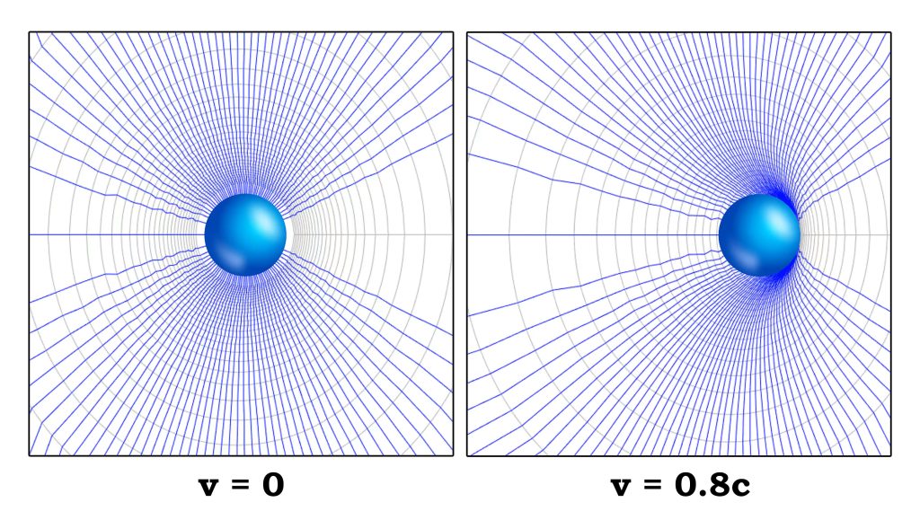
To plot the potential and displacement, we can convert eqn(12) of potential into two dimensional equation for the sake of simplicity in visualization. We can replace z as x as we can visualize moving in x direction and remove the actual x part. Also the equation is with respect to moving frame. To get the proper field picture, we can transform the x-axis into the stationary from using x → x – vt. Then we can ploy y as:
Following are the plot of potential (in gray) and displacement (in blue) for the the charged object when the v =0 and when v = 0.8c.
You can clearly see when the speed approach that of light, the field starts to distort as they don’t get enough time to realign, hence compressing the aether. Following is a short visualization with animation.
The magnetic field intensity H can be now derived from D using eqn(3), as:\large \overrightarrow{H}=\frac{Q}{4 \pi}\frac{1}{\sqrt{1-\frac{v_{z}^{2}}{c^{2}}}}\frac{v_{z}}{ (x^{2}+y^{2}+\frac{1}{1-\frac{v_{z}^2}{c^2}}z^{2})^{\frac{3}{2}}}(-y\hat{i}+x\hat{j})
The magnetic field intensity H can be now derived from D using eqn(3), as:\small \overrightarrow{H}=\frac{Q}{4 \pi}\frac{1}{\sqrt{1-\frac{v_{z}^{2}}{c^{2}}}}\frac{v_{z}}{ (x^{2}+y^{2}+\frac{1}{1-\frac{v_{z}^2}{c^2}}z^{2})^{\frac{3}{2}}}(-y\hat{i}+x\hat{j})
The magnetic energy per unit volume is given from eqn(1) as \large \frac{\mu}{2}\left| H \right|^{2}=\frac{\mu Q^2}{32 \pi^{2}}\frac{1}{(1-\frac{v_{z}^{2}}{c^{2}})}\frac{v_{z}^{2}(x^2+y^{2})}{ (x^{2}+y^{2}+\frac{1}{1-\frac{v_{z}^2}{c^2}}z^{2})^{3}}
The magnetic energy per unit volume is given from eqn(1) as \small \frac{\mu}{2}\left| H \right|^{2}=\frac{\mu Q^2}{32 \pi^{2}}\frac{1}{(1-\frac{v_{z}^{2}}{c^{2}})}\frac{v_{z}^{2}(x^2+y^{2})}{ (x^{2}+y^{2}+\frac{1}{1-\frac{v_{z}^2}{c^2}}z^{2})^{3}}
Converting the kinetic energy per unit volume into spherical coordinate we get:\large \frac{\mu Q^2}{32 \pi^{2}}\frac{v_{z}^{2}}{(1-\frac{v_{z}^{2}}{c^{2}})}\frac{sin^2\theta}{ r^{4}(sin^{2}\theta+\frac{1}{1-\frac{v_{z}^2}{c^2}}cos^{2}\theta)^{3}}
To calculate the total kinetic energy we need to integrate the above expression for the entire space after the sphere surface.\begin{align*}\large K.E &= \large\frac{\mu Q^2}{32 \pi^{2}}\frac{v_{z}^{2}}{(1-\frac{v_{z}^{2}}{c^{2}})}\int_{0}^{2 \pi }\int_{0}^{\pi}\int_{a}^{\infty }\frac{sin^2\theta}{ r^{4}(sin^{2}\theta+\frac{1}{1-\frac{v_{z}^2}{c^2}}cos^{2}\theta)^{3}} r^{2}sin\theta \partial \theta \partial \phi \\
&= \large\frac{\mu Q^2}{16 \pi}\frac{v_{z}^{2}}{(1-\frac{v_{z}^{2}}{c^{2}})}\int_{0}^{\pi}\int_{a}^{\infty }\frac{sin^3\theta}{ r^{2}(sin^{2}\theta+\frac{1}{1-\frac{v_{z}^2}{c^2}}cos^{2}\theta)^{3}} \partial \theta \\
&= \large\frac{\mu Q^2}{16 \pi a}\frac{v_{z}^{2}}{(1-\frac{v_{z}^{2}}{c^{2}})}\int_{0}^{\pi}\frac{sin^3\theta}{ (sin^{2}\theta+\frac{1}{1-\frac{v_{z}^2}{c^2}}cos^{2}\theta)^{3}} \partial \theta \\
&= \large\frac{\mu Q^2}{16 \pi a}\frac{v_{z}^{2}}{(1-\frac{v_{z}^{2}}{c^{2}})}\int_{0}^{\pi}\frac{sin^3\theta}{ (1+\frac{v_{z}^2}{c^{2}-v_{z}^{2}}cos^{2}\theta)^{3}} \partial \theta
\end{align*}
To calculate the total kinetic energy we need to integrate the above expression for the entire space after the sphere surface.\begin{align*}\small K.E &= \tiny \frac{\mu Q^2}{32 \pi^{2}}\frac{v_{z}^{2}}{(1-\frac{v_{z}^{2}}{c^{2}})} \small \int_{0}^{2 \pi }\int_{0}^{\pi}\int_{a}^{\infty }\tiny \frac{sin^2\theta}{ r^{4}(sin^{2}\theta+\frac{1}{1-\frac{v_{z}^2}{c^2}}cos^{2}\theta)^{3}} r^{2}sin\theta \partial \theta \partial \phi \\
&= \small \frac{\mu Q^2}{16 \pi}\frac{v_{z}^{2}}{(1-\frac{v_{z}^{2}}{c^{2}})}\int_{0}^{\pi}\int_{a}^{\infty }\tiny \frac{sin^3\theta}{ r^{2}(sin^{2}\theta+\frac{1}{1-\frac{v_{z}^2}{c^2}}cos^{2}\theta)^{3}} \small \partial \theta \\
&= \small \frac{\mu Q^2}{16 \pi a}\frac{v_{z}^{2}}{(1-\frac{v_{z}^{2}}{c^{2}})}\int_{0}^{\pi}\frac{sin^3\theta}{ (sin^{2}\theta+\frac{1}{1-\frac{v_{z}^2}{c^2}}cos^{2}\theta)^{3}} \partial \theta \\
&= \small \frac{\mu Q^2}{16 \pi a}\frac{v_{z}^{2}}{(1-\frac{v_{z}^{2}}{c^{2}})}\int_{0}^{\pi}\frac{sin^3\theta}{ (1+\frac{v_{z}^2}{c^{2}-v_{z}^{2}}cos^{2}\theta)^{3}} \partial \theta
\end{align*}
To solve the above integral, let’s set:cos\theta = u \\
Hence,\: sin\theta\: \partial\theta = - \partial u
Now the integral becomes:\begin{align*}\large K.E &=\large\frac{\mu Q^2}{16 \pi a}\frac{v_{z}^{2}}{(1-\frac{v_{z}^{2}}{c^{2}})}\int_{1}^{-1}\frac{u^{2} - 1}{ (1+\frac{v_{z}^2}{c^{2}-v_{z}^{2}}u^{2})^{3}} \partial u
\end{align*}
Now the integral becomes:\begin{align*}\small K.E &=\small \frac{\mu Q^2}{16 \pi a}\frac{v_{z}^{2}}{(1-\frac{v_{z}^{2}}{c^{2}})}\int_{1}^{-1}\frac{u^{2} - 1}{ (1+\frac{v_{z}^2}{c^{2}-v_{z}^{2}}u^{2})^{3}} \partial u
\end{align*}
Now again set:\begin{align*}\large \frac{v_{z}}{\sqrt{c^{2}-v_{z}^{2}}}u = tan \psi \\
so, \partial u = \frac{\sqrt{c^{2}-v_{z}^{2}}}{v_{z}}sec^{2}\psi \partial \psi
\end{align*}
So now the total kinetic energy of the system is the sum of mechanical and magnetic energy, which is:\large K.E = \large K.E_{M} + K.E_{E} \\
\begin{align*}\large \frac{1}{2}Mv_{z}^{2} &= \small \frac{1}{2}mv_{z}^{2} + \frac{\mu Q^2}{16 \pi a}\frac{v_{z}c^{2}}{\sqrt{c^{2}-v_{z}^{2}}}\left\{v_{2}(1 - \frac{c^{2}}{4v_{z}^{2}}) + \frac{1}{2}sin 2v_{2}(1+\frac{c^2}{4v_{z}^{2}}cos2v_{2})\right\} \\
&= \small \frac{1}{2}v_{z}^{2}\left[ m + \frac{\mu Q^2}{8 \pi a}\frac{c^{2}}{v_{z}\sqrt{c^{2}-v_{z}^{2}}}\left\{v_{2}(1 - \frac{c^{2}}{4v_{z}^{2}}) + \frac{1}{2}sin 2v_{2}(1+\frac{c^2}{4v_{z}^{2}}cos2v_{2})\right\}\right]
\end{align*} \\
or, \large M = m + \small \frac{\mu Q^2}{8 \pi a}\frac{c^{2}}{v_{z}\sqrt{c^{2}-v_{z}^{2}}}\left\{v_{2}(1 - \frac{c^{2}}{4v_{z}^{2}}) + \frac{1}{2}sin 2v_{2}(1+\frac{c^2}{4v_{z}^{2}}cos2v_{2})\right\}
So now the total kinetic energy of the system is the sum of mechanical and magnetic energy, which is:\large K.E = \large K.E_{M} + K.E_{E} \\
\begin{align*}\small \frac{1}{2}Mv_{z}^{2} &= \small \frac{1}{2}mv_{z}^{2} + \frac{\mu Q^2}{16 \pi a}\frac{v_{z}c^{2}}{\sqrt{c^{2}-v_{z}^{2}}} \\
& \small \left\{v_{2}(1 - \frac{c^{2}}{4v_{z}^{2}}) + \frac{1}{2}sin 2v_{2}(1+\frac{c^2}{4v_{z}^{2}}cos2v_{2})\right\} \\
&= \small \frac{1}{2}v_{z}^{2}\large [ \small m + \frac{\mu Q^2}{8 \pi a}\frac{c^{2}}{v_{z}\sqrt{c^{2}-v_{z}^{2}}} \\ & \small \left\{v_{2}(1 - \frac{c^{2}}{4v_{z}^{2}}) + \frac{1}{2}sin 2v_{2}(1+\frac{c^2}{4v_{z}^{2}}cos2v_{2})\right\} \large ]
\end{align*} \\
\begin{align*}or,\:\:\: \small M &= m + \small \frac{\mu Q^2}{8 \pi a}\frac{c^{2}}{v_{z}\sqrt{c^{2}-v_{z}^{2}}} \\ & \small \left\{v_{2}(1 - \frac{c^{2}}{4v_{z}^{2}}) + \frac{1}{2}sin 2v_{2}(1+\frac{c^2}{4v_{z}^{2}}cos2v_{2})\right\}\end{align*}
So the mass of the object is increased by amount:\small \frac{\mu Q^2}{8 \pi a}\frac{c^{2}}{v_{z}\sqrt{c^{2}-v_{z}^{2}}}\left\{v_{2}(1 - \frac{c^{2}}{4v_{z}^{2}}) + \frac{1}{2}sin 2v_{2}(1+\frac{c^2}{4v_{z}^{2}}cos2v_{2})\right\}
So the mass of the object is increased by amount:\begin{align*} & \small \frac{\mu Q^2}{8 \pi a}\frac{c^{2}}{v_{z}\sqrt{c^{2}-v_{z}^{2}}} \\ & \large [ \small v_{2}(1 - \frac{c^{2}}{4v_{z}^{2}}) + \frac{1}{2}sin 2v_{2}(1+\frac{c^2}{4v_{z}^{2}}cos2v_{2}) \large ]\end{align*}
By evaluating the above extra mass quantity by converting factors sin2v2 and cos2v2 in terms of tan and evaluate it using the value of v2, we get:
You can see if velocity approaches to that of speed of light (vz = c), the mass tends to increase to infinity. So it’s velocity will remain constant. So its impossible to increase the velocity of a charged boy more than that of the speed of light in this scenario.
If speed of the object is very very less than that of light,\begin{align*} & \small \text{the factor} \:\: tan^{-1} \frac{v_{z}}{\sqrt{c^{2}-v_{z}^{2}}} \text{can be approximated as:} \\
\small &\simeq v_{z}(c^{2}-v_{z}^{2})^{\frac{-1}{2}} - \frac{v_{z}^{3}}{3}(c^{2}-v_{z}^{2})^{\frac{-1}{6}} \:\:\:\:\:\:\: \tiny \text{[Using Maclaurin Series]} \\
\small &\simeq \frac{v_{z}}{c}\left( 1 -\frac{v_{z}^{2}}{c^{2}} \right) ^{-\frac{1}{2}} -\frac{v_{z}^{3}}{3c^{3}}\left( 1 -\frac{v_{z}^{2}}{c^{2}} \right) ^{-\frac{1}{6}} \\
\small &\simeq \frac{v_{z}}{c} - \frac{v_{z}^{3}}{3c^{3}}\left( 1 +\frac{v_{z}^{2}}{6c^{2}} \right) \:\: \tiny \text{[dropping the factor } \frac{v_{z}^{2}}{c^{2}} \text{ in the first term and using Binomial expansion for the second]}
\end{align*}
If speed of the object is very very less than that of light,\begin{align*} & \small \text{the factor} \:\: tan^{-1} \frac{v_{z}}{\sqrt{c^{2}-v_{z}^{2}}} \text{can be approximated as:} \\
\small &\simeq v_{z}(c^{2}-v_{z}^{2})^{\frac{-1}{2}} - \frac{v_{z}^{3}}{3}(c^{2}-v_{z}^{2})^{\frac{-1}{6}} \:\: \tiny \text{[Using Maclaurin Series]} \\
\small &\simeq \frac{v_{z}}{c}\left( 1 -\frac{v_{z}^{2}}{c^{2}} \right) ^{-\frac{1}{2}} -\frac{v_{z}^{3}}{3c^{3}}\left( 1 -\frac{v_{z}^{2}}{c^{2}} \right) ^{-\frac{1}{6}} \\
\small &\simeq \frac{v_{z}}{c} - \frac{v_{z}^{3}}{3c^{3}}\left( 1 +\frac{v_{z}^{2}}{6c^{2}} \right) \\
& \tiny \text{[dropping the factor } \frac{v_{z}^{2}}{c^{2}} \text{ in the first term and using Binomial expansion for the second]}
\end{align*}
So the increased mass quantity becomes\small \frac{\mu Q^2}{8 \pi a}\frac{c^{2}}{v_{z}\sqrt{c^{2}-v_{z}^{2}}}\left [\left\{\frac{v_{z}}{c} - \frac{v_{z}^{3}}{3c^{3}}\left( 1 +\frac{v_{z}^{2}}{6c^{2}} \right) \right\}\left(\frac{4v_{z}^{2} -c^{2}}{4v_{z}^{2}}\right) + \frac{(2v_{z}^{2}+c^{2})}{4v_{z}c^{2}}\sqrt{c^{2}-v_{z}^{2}}\right ] \\
\begin{align*}
&= \small \frac{\mu Q^2}{8 \pi a}\frac{1}{4v_{z}^{2}\sqrt{1-\frac{v_{z}^{2}}{c^{2}}}}\left[(1 -\frac{v_{z}^{2}}{3c^{2}}-\frac{v_{z}^{4}}{18c^{4}})(4v_{z}^{2}-c^{2}) +(2v_{z}^{2}+c^{2})\sqrt{1-\frac{v_{z}^{2}}{c^{2}}} \right] \\
& \simeq \small \frac{\mu Q^2}{8 \pi a}\frac{1}{4v_{z}^{2}}\left[ 4v_{z}^{2} -\frac{4v_{z}^{4}}{3c^{2}}-\frac{2v_{z}^{6}}{9c^{4}}-c^{2} + \frac{v_{z}^{2}}{3}+\frac{v_{z}^{4}}{18c^{2}} + 2v_{z}^{2} + c^{2} \right] \: \: \: \tiny \text{[By dropping the negligible factor }\sqrt{1-\frac{v_{z}^{2}}{c^{2}}} \text{ ]} \\
&= \frac{\mu}{2 \pi}\frac{Q^{2}}{a}\frac{1}{16}\left[ \frac{19}{3} -\frac{69v_{z}^{2}}{54c^{2}} - \frac{2v_{z}^{4}}{9c^{4}} \right] \\
& \simeq \frac{\mu}{2 \pi}\frac{Q^{2}}{3a}\frac{19}{16} \tiny \:\:\:\:\:\:\:\:\:\:\:\: \text{[Dropping the negligible last two terms]} \\
& \simeq \frac{\mu}{2 \pi}\frac{Q^{2}}{3a}\tiny \:\:\:\:\:\:\:\:\:\:\:\: \text{[As the factor } \frac{19}{16} = 1.18 \text{ is small and will be getting smaller if more terms of approximation is used. So dropped]}
\end{align*}
So the increased mass quantity becomes\begin{align*} & \small \frac{\mu Q^2}{8 \pi a}\frac{c^{2}}{v_{z}\sqrt{c^{2}-v_{z}^{2}}} \large[ \\
& \:\:\:\:\:\:\: \small \left\{\frac{v_{z}}{c} - \frac{v_{z}^{3}}{3c^{3}}\left( 1 +\frac{v_{z}^{2}}{6c^{2}} \right) \right\}\left(\frac{4v_{z}^{2} -c^{2}}{4v_{z}^{2}}\right) \\
& \:\:\:\:\:\:\: \small + \frac{(2v_{z}^{2}+c^{2})}{4v_{z}c^{2}}\sqrt{c^{2}-v_{z}^{2}} \large \: ] \\
&= \small \frac{\mu Q^2}{8 \pi a}\frac{1}{4v_{z}^{2}\sqrt{1-\frac{v_{z}^{2}}{c^{2}}}}\large [ \small (1 -\frac{v_{z}^{2}}{3c^{2}}-\frac{v_{z}^{4}}{18c^{4}})(4v_{z}^{2}-c^{2}) \\
& \:\:\:\:\:\:\: \small +(2v_{z}^{2}+c^{2})\sqrt{1-\frac{v_{z}^{2}}{c^{2}}} \large \: ] \\
& \simeq \small \frac{\mu Q^2}{8 \pi a}\frac{1}{4v_{z}^{2}}\large [ \small 4v_{z}^{2} -\frac{4v_{z}^{4}}{3c^{2}}-\frac{2v_{z}^{6}}{9c^{4}}-c^{2} + \frac{v_{z}^{2}}{3} \\
& \small \:\:\:\:\:\:\: +\frac{v_{z}^{4}}{18c^{2}} + 2v_{z}^{2} + c^{2} \large \: ] \: \: \: \tiny \text{[By dropping the negligible factor }\sqrt{1-\frac{v_{z}^{2}}{c^{2}}} \text{ ]} \\
&= \frac{\mu}{2 \pi}\frac{Q^{2}}{a}\frac{1}{16}\left[ \frac{19}{3} -\frac{69v_{z}^{2}}{54c^{2}} - \frac{2v_{z}^{4}}{9c^{4}} \right] \\
& \simeq \frac{\mu}{2 \pi}\frac{Q^{2}}{3a}\frac{19}{16} \tiny \:\:\:\:\:\:\:\: \text{[Dropping the negligible last two terms]} \\
& \simeq \frac{\mu}{2 \pi}\frac{Q^{2}}{3a} \:\:\:\: \tiny \text{[As the factor } \frac{19}{16} = 1.18 \text{ is small and will be getting smaller } \\
& \:\:\:\:\:\:\:\: \:\:\:\:\:\:\:\: \:\:\:\:\:\:\:\: \tiny \text{if more terms of approximation is used. So dropped]}
\end{align*}
This is the same factor which we obtained in our pervious analysis without considering any field distortion.
So does this prove that speed of light is the maximum limit to any charged bodies? And what about neutral bodies?
Well that’s not the case. The limit of speed of light is for very limiting condition like the one mentioned here. There are many ways to overcome it. Unfortunately this very specific case for electrodynamics of moving bodies is being misinterpreted and generalized into erroneous theories like relativity without any physical medium.
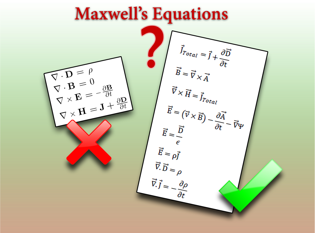
Why you believe he derived only 4 equations? Just because your textbook and consensus says? Why not read the original papers and books of Maxwell itself. They are all rotting in archive.org.
For your kind information the so-called Maxwell’s equation used today are actually Heaviside equations.
Maxwell compiled 8 sets of quaternion equations form the experimental findings of Faraday, Gauss, Ampere, Ohm, Weber, Helmholtz, Kohlrausch etc. and converted them into symbolic calculation methods, in his paper A Dynamic Theory of Electromagnetic Field.
Maxwell’s only original contribution is displacement current.
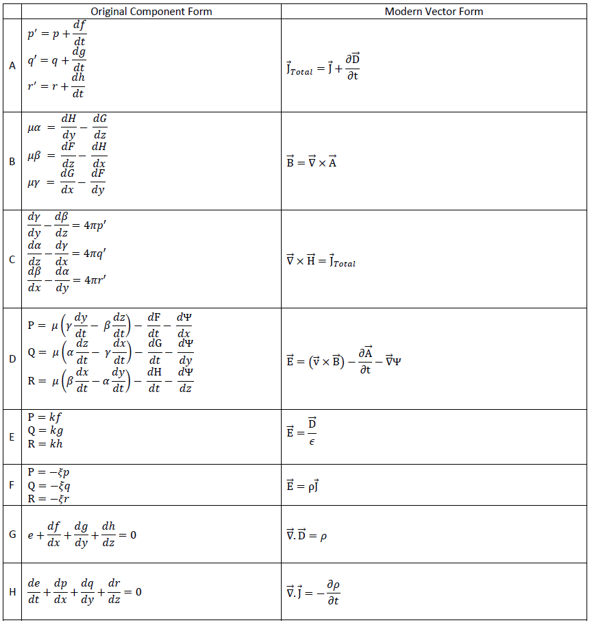
If you expand the vector into component form, there will be total twenty equations involving twenty variable quantities, as you can see in below.
As vector notation were not there at his time, hence all vector equations are written in individual component form.
He thought that certain phenomena in electricity and magnetism lead to the same conclusion as those of optics, namely, that there is an aethereal medium pervading all bodies, and modified only in degree by their presence; that the parts of this medium are capable of being set in motion by electric currents and magnets; that this motion is communicated from one part of the medium to another by forces arising from the connections of those parts; that under the action of these forces there is a certain yielding depending on the elasticity of these connections; and that therefore energy in two different forms may exist in the medium, the one form being the actual energy of motion of its parts, and the other being the potential energy stored up in the connections, in virtue of their elasticity.
We know that when an electric current is established in a conducting circuit, the neighboring part of field is characterized by certain magnetic properties, and that if two circuits are in the field, the magnetic properties of the field due to the two currents are combined. Thus each part of the field is in connection with both currents, and the two currents are put in connection with each other in virtue of their connection with the magnetization of the field.
The first result of this connection that I propose to examine, is the induction of one current by another, and by the motion of conductors in the field.
The second result, which is deduced from this, is the mechanical action between conductors carrying currents. This phenomenon was deduced by Helmholtz and W Thomson. Maxwell followed the reverse order and deduced the mechanical action from the law of induction.
He then applied the phenomena of induction and attraction of currents to the exploration of the electromagnetic field, and the laying down system of lines of magnetic force which indicate its magnetic properties.
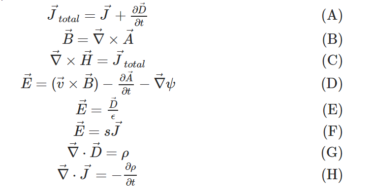
He used 8 sets of question A-H as I mentioned at the beginning. They represents following: (A) The relation between electric displacement, true condition, and total current, compounded of both. (B) The relation between the lines of magnetic force and the inductive coefficients of a circuit, as already deducted from the laws of induction. (C) The relation between the strength of a current and its magnetic effects, according to the electromagnetic system of measurement. (D) The value of the electromotive force in a body, as arising from the motion of the body in the field, the alteration of the field itself, and the variation of electric potential from one part of the field to another. (E) The relation between an electric displacement, and electromotive force which produced it. (F) The relation between an electric current, and the electromotive force which produces it. (G) The relation between the amount of free electricity at any point, and the electric displacements in the neighborhood. (H) The relation between the increase or diminution of free electricity and the electric currents in the neighborhood.
He determined the mechanical force acting 1st, on a movable conductor carrying an electric current; 2ndly, on a magnetic pole; 3rdly, on an electrified body.
The last result, namely, the mechanical force acting on an electrified body, gives rise to an independent method of electrical measurement founded on its electrostatic effects. The relation between the units employed in the two methods is shown to depend on what he called the “electric elasticity” (now reciprocal of permittivity) of the medium, and to be a velocity, which has been experimentally determined by Weber and Kohlrausch.
The displacement current leads to the possibility of wave propagation in free space. This also lead to the possibility of electric lines of force forming closed loops, independent of any charge. This evolves the way of primitive thinking that current is not something inside the conductor like water in a pipe, rather all around the space surrounding it. Unfortunately today this thinking has taken a backseat.
It’s Oliver Heaviside who invented his vector calculus to downgrade and simplify Maxwell equations into 4 vector form which we “incorrectly” address as Maxwell’s equations.
Heaviside gave birth to practical electrical engineering by solving transatlantic cable problem. He wanted to establish telephone lines. So he removed the scalar and vector potential and force equation from Maxwell original sets of equation to make it more practical, also limited.
Potentials can lead to realization of longitudinal waves also which would be considered impossible as per Heaviside equation.
Unfortunately, due to academic laziness, these truncated equations are still dominating in industry and claimed as Maxwell’s.
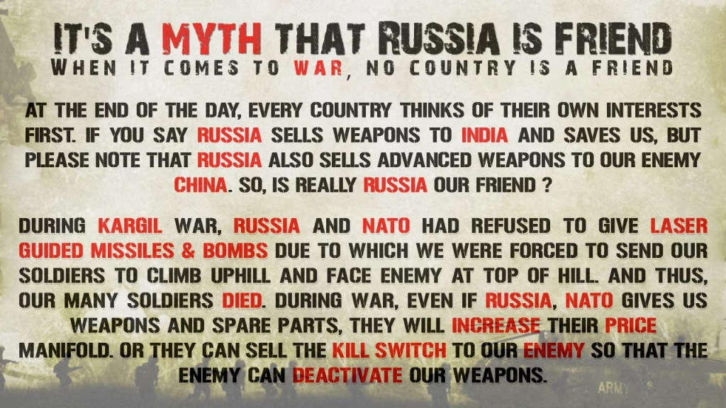
In Geopolitics, There are Only INTERESTS, NO FRIENDS.
It’s a myth that Russia is a friend. When it comes to War, no country is a friend. At the end of the day, every country thinks of their own interests first. If you say Russia sells weapons to India and will always save us, but please note that Russia also sells advanced weapons to our enemy China.
Russia and China are revitalising defence ties at a time when relations of both with the U.S. have run into rough waters
Israel supplied us laser guided bombs and Bofors at a later stage when other countries did not give us these weapons. And it is well known that NATO and Israel are under big boss, US influence. During 1999 Kargil war, Russia and NATO had refused to give laser guided missiles and bombs, due to which we were forced to send our soldiers to climb up hill and face enemy at the top of the hill and thus our many soldiers died.
During War, even if Russia, NATO gives us weapons and spare parts, they will increase their price manifold. Or they can sell the kill switch (radio switch) to our enemy so that the enemy can deactivate our weapons.
See the issue with high altitude due to lack of LGB technology and how Mirage 2000 LGB kit parts were supplied with incorrect parts due to India’s Pokhran II test which Russia didn’t like.